Technical Work: Sequential Dijkstra

One of the pathfinding algorithms that i am aiming to compare against the parallel diffusion implementation is a sequential and parallel implementation of Dijkstra. This post will provide a background to Dijkstra's algorithm and an overview of the sequential implementation.

Background

Dijkstra's algorithim was first presented by Edsger Dijkstra in 1959 as a path finding algorithm that solves the single-source shortest path problem for a non-negative weighted graph. Nodes in the graph can represent either a 2-dimensional grid or points in 3D space. In many examples it is often used to find paths between connected cities where each city is represented as a node in the graph and each edge is a road with an associated cost. For a given source node dijkstra is able to find the lowest cost path between that node and every other node in the graph.

Non-negative weighted graph of connected cities.

The algorithm itself works by assigning a distance value to each node in the graph,  setting the value for our source node to zero and every other node to infinity. Initially we mark all nodes as unvisited and store them in a priority queue called the unvisited set. For our current source node we look at all of its unvisited neighbours and calculate the distance from our current node to the neighbouring node. For example, in figure 1 above if our current node was Tranent and we were looking at neighbour Musselburgh our distance would be 4. If this distance is less than our previous shortest path we add our current node to a shortest path tree which we can later use to backtrack a path to the source node. Once we have looked at all the neighbouring nodes we remove our current node from the unvisited set and it will not be checked again. Next we set our current node to the node with the smallest distance in the unvisited set and repeat the process with this nodes neighbours until all the nodes have been visited. At this point our shortest path graph will now contain all of the lowest cost paths from our source node to every other node, we can then perform a depth-first search over this graph to find a path from any node to the source.

Sequential Implementation

Our sequential implementation initially reads in a map from a .CSV file containing the costs of each tile in a 2D grid.

Example cost Grid

From this we build up a non-negative weighted graph of connected nodes which is stored in a 2 dimensional vector. Each node in the graph has an associated id, cost and list of its connected neighbours. A node is connected to other nodes based on the 8 surrounding nodes in the cost grid, for each neighbour diagonal to a node its cost is increased slightly. 

Once we have the node graph set up we are able to run our dijkstra algorithm on the graph. Our method takes in the x and y co-ordinates of the source node, a vector that will be used to store the minimum distance of each node to the source and a vector containing the previous position of the node closest to the source. 

Run the Dijkstra algorithm

Within the dijkstra method we create a priority queue to store all our unvisited nodes, we use a priority queue as it allows easy insertion and deletion of nodes and keeps our nodes ordered with the lowest cost node first in the queue. We then add our source node to the queue setting its initial cost to zero. 

While there a still nodes remaining unvisited in the queue we perform the following actions. 

1. Remove the node with the lowest cost from the queue.
2. Visit each of the nodes neighbours
• Calculate the cost of passing through this neighbour
• If this cost is less than our previously calculated cost
• Set the new cost to our new minimum cost
• set the parent of this neighbour to the current node being checked
• add the neighbour to the queue with the new calculated cost
3. Repeat step 1 if queue is not empty.

Once the queue is empty all of our nodes will have been visited and our previous vector will contain a shortest path tree for all of the nodes to the source. At this stage we can backtrack a path from any node to the source node. 

Our backtrack method takes a given goal node and using the shortest path tree backtracks through each of the nodes parent nodes adding them to a list until it reaches the original source node. 

At this point we now have a list containing all the nodes in a path between the original source node and the specified goal, this is then written to a .csv file so that we may view the path.

Examples

In each of these examples we read in a 32x32 cost grid to create our node graph from and perform our pathfinding to find a path between two points in the grid. The length of a path is defined as the number of nodes in the path and the cost of a path is the total cost of all the nodes.

In the first example above we have essentially an empty cost grid where every tiles value is 1 and we are trying to find a path between the two green points.

 

Above we can see that as would typically be expected the best and shortest path between the two points would be to move in a straight line. the length of the path is 30 and the cost of this path is 29. 

Above we have added a small lake into the center of our map, the cost of passing through a tile with water in it is 100.

As we can see our path has avoided the water, choosing instead to simply go around rather than through. This is due to the fact that moving through the water would incur a large cost and as such is not the shortest path. The length of this path is 30 and the cost is 43 (Moving diagonally has an additional cost).

This time we have added an old rickety bridge across the water with a cost of 25 to cross. 

While costing less to cross than water, crossing the old bridge would still not be the shortest path between our two points and as such our path has chosen to avoid it and go around the water. This path has a length of 30 and a cost of 43.

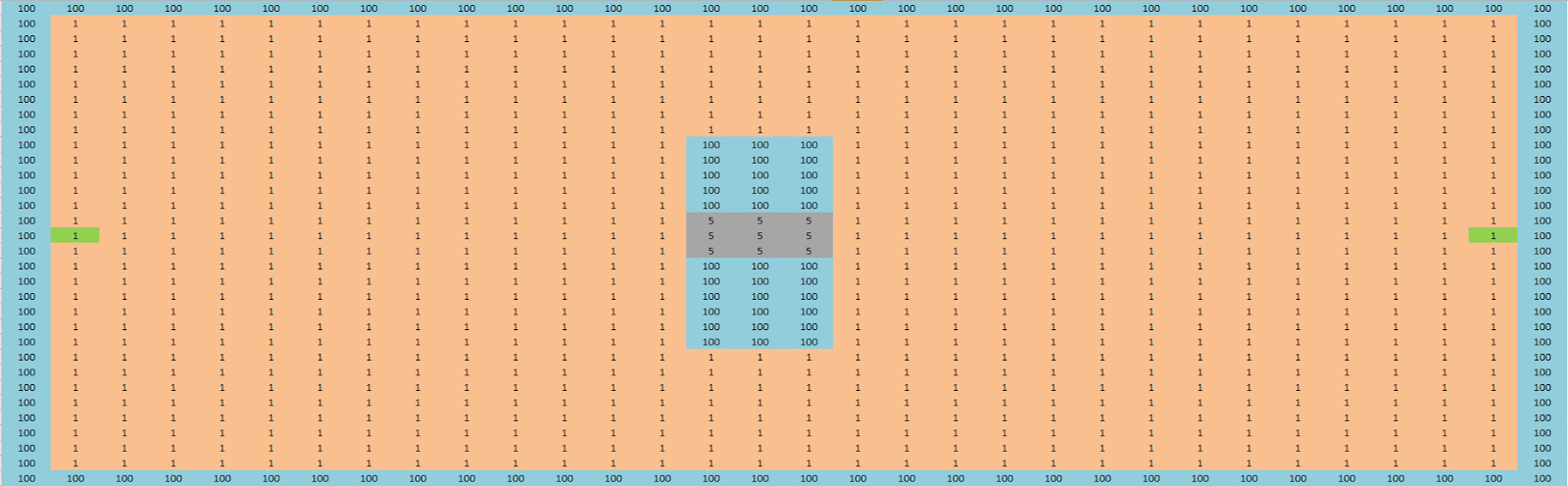
Our bridge has been upgraded to a super strong concrete bridge made by the finest engineers and now only has a cost of 5 to cross. 

As our bridge is now more stable and has a lower cost to cross, the shortest path between our two points is now to take the bridge rather than going around and as such our path length is 30 with a cost of 41.