Frontier Set Visualizations

The following images show which nodes are added to the frontier set at the same time and processed in parallel for the GPU Dijkstra application. Colours closer to red are processed first with colours closer to green being done last. Areas of the same colour are processed in parallel.

Map 1

Map 2

Map 3

Map 4

Map 5

Map 6

What is interesting here is that the areas in the map with a higher terrain cost are all processed at the same time, after all the areas of lower cost have been processed resulting in our heat maps looking very similar to the actual maps.

This behaviour appears to make sense based upon the way that the Frontier set selection method works. As at each iteration we select all nodes in the queue which have a cost of less than the minimum cost + 1. This means that all the low cost areas will be processed first with high cost areas being processed last as we have shown through the tests and the visualizations.

Scattered Terrain: Diffusion vs Dijkstra

Both diffusion and dijkstra have been tested on larger maps with varying terrain. These maps are 256X256 and each has a different percentage of the map covered with terrain. Terrain costs are represented by a random value between 1 and 10 for dijkstra and 0 and 1 for diffusion. In the images bellow terrain is represented by the red areas. Paths are represented by the blue tiles.

0% Terrain

25% Scattered Terrain

50% Scattered Terrain

75% Scattered Terrain

100% Scattered Terrain

25% Centred Terrain

50% Centred Terrain

75% Centred Terrain

100% Centred Terrain

25% Split Terrain

50% Split Terrain

75% Split Terrain

100% Split Terrain

Looking at the graphs above it is interesting to see that for all the maps diffusion performs the same regardless of how much terrain there is in the map and where the terrain is in the map taking 11ms to diffuse the values and find path.

Looking at Dijkstra however for each of the sets of maps we can see that as the amount of terrain in the map increases so does the time it takes to find a path.

Looking at the line graph above we can also see that the position of the terrain in the maps also effects the time taken by dijkstra to find the path. the more scattered the terrain the longer Dijkstra takes to find a path? although this could be due to the fact that there is less terrain? - more likely this?

Visualization of nodes added to frontier set

Each colour represents the iteration of the outer loop that the node was added to the frontier set.

Tests to run

Run both dijkstra and diffusion for maps with varying terrain, use larger maps with different portions covered with terrain. i.e 25% 50% 75% and have terrain spread out vs grouped together See how this effects the time taken and the nodes added to the frontier set.

Run each for an average of 10 times,

create the maps and store them in a .CSV file so the same maps can be used each time.

Nodes added to the frontier set each iteration

number of nodes added to frontier set each iteration increase by 2, ascending in odd numbers to n + n -1 where n is the size of the grid. the sum of the nodes added each iteration for all iterations is equal to n*n.

Iteration	Nodes In Frontier
0	1
1	3
2	5
3	7
4	9
5	11
6	13
7	15
8	17
9	19
10	21
11	23
12	25
13	27
14	29
15	31
16	33
17	35
18	37
19	39
20	41
21	43
22	45
23	47
24	49
25	51
26	53
27	55
28	57
29	59
30	61
31	63

Parallel Dijkstra

Map	Time
32X32	3.46784
64X64	6.455913
128X128	13.38988
256X256	28.1704
512X512	72.76363
1024X1024	278.0663
2048X2048	1729.728
4096X4096	10725.9
8192X8192	80471.69

Internship Plan - 14/07/14

1. Explore path search algorithms using CUDA Dynamic Parallelism 
1. Cut down Honours Project
2. Extend Tests
3. Weighted vs Non-Weighted
2. Fine grained dynamic parallelism support for Dijkstra
1. Do more practical work
3. Examine Frontier Sets
4. Parallelise A*
5. Compare to Ortega-Arranz Implementation
6. Read Requirements of Journals
7. Plan out what the paper will look like

Possible Journals and Conferences

1. High Performance Computing & Simulation
2. Concurrency and Computation, Practice and Experience
3. GPU Gems
4. GTC

Poster Presentation 9th April 2014

The video below is a small demo which shows the difference in paths between diffusion and dijkstra. The green paths represent diffusion while the purple paths represent dijkstra. 

Meetings: Monday 24th March 2014

Discussed the poster presentation and what needs to be included in the poster. The aim is to have an initial draft by Monday 31st March.

Also need to revise the initial questions outlined during the background. Possible questions are.

1. Find a suitable algorithm for path finding on the GPU.
2. Quantify in terms of
     a) speed
     b) Layout of path - scalability
     c) trade-off : Speed vs Path style
3. What contributes to the GPU - Mapping of algorithms to the GPU

Also need a section for contributions.

Meetings: Monday 17th March

Discussed the results obtained from last weeks experiments and concluded that all the implementation, results and testing have all been completed. The remainder of the project will be focused on the write up and the poster session.

Discussed that it should be possible to use the coursework for computational intelligence to show a robot moving through the maze using collaborative diffusion.

Parallel Dijkstra

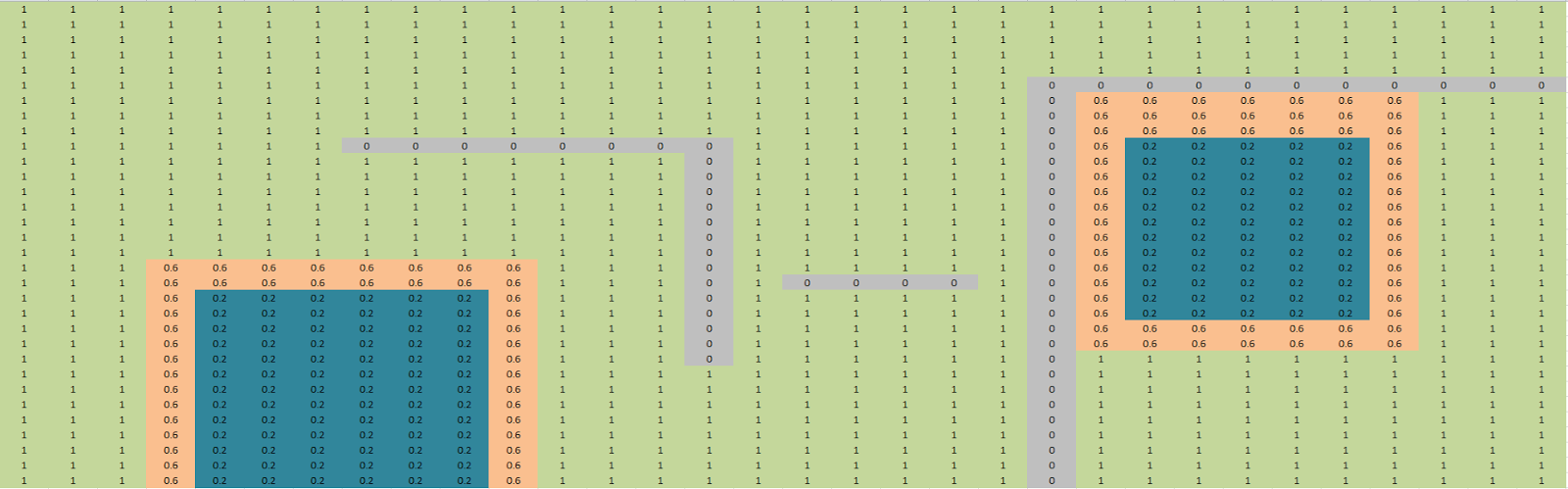
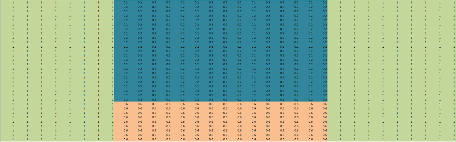
Map 1

Map 2

Map 3

Map 4

Map 5

Map 6

The parallel dijkstra application has been tested on the original 5 maps used on the sequential dijkstra and the diffusion applications. For each map the parallel version found the same path as the sequential version.

Map	Parallel (ms)	Sequential (ms)
1	8.42	0.97
2	33.82	1.01
3	40.78	1.05
4	55.87	1.00
5	18.58	0.64
6	51.91	0.95

Time for each map

Looking at the times taken for each map we can see quite a large difference between the parallel and sequential times. Even between the differing maps there is a large variation for just the parallel times, whereas the sequential times remain fairly consistent at around 1ms.

This is due to main while loop of the dijkstra application, where loop until the queue is empty and all nodes have been evaluated. 

Map	Parallel	Sequential
1	32	1024
2	132	1024
3	159	1024
4	219	1024
5	72	701
6	203	1024

 Iterations to evaluate all nodes in queue

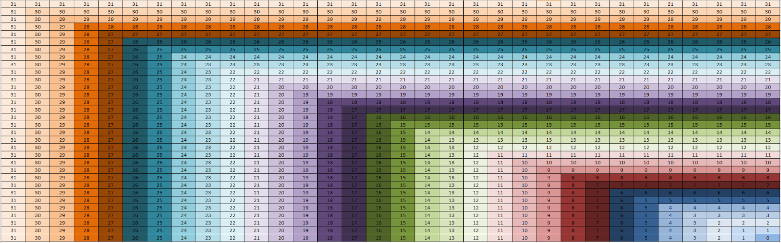
Looking at the number of iterations needed in the sequential version we can see that it remains pretty much consistent taking 1024 iterations to evaluate each node in the queue, interestingly this is the total number of nodes added to the queue as we have 32*32 nodes and we evaluate each one. (Note: map 5 we only add 701 nodes to the queue as a number of nodes are blocked.)

However looking at the parallel version the number of iterations jumps between 32 and 219 for the differing map sizes. This is due to the frontier function and the way in which the parallel application works. 

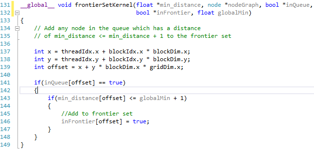
The parallel application determines which nodes in the queue can be settled at the same time and adds them to the frontier set. Any node in the queue which has a distance of less than the minimum distance + 1 will be added to the queue. 

In each of the maps a lot of nodes have varying costs, these varying costs between neighbours will effect which nodes in the queue can be added to the frontier set and settled at the same time, the more variation between nodes the more iterations it will take to find the path. In each instance the worst case should be 1024 iterations for the 32x32 grid.

This also helps to explain why we see a speed up for the larger graph sizes, while the CPU is able to process 1024 iterations faster than the GPU can handle 32; for the large graph sizes the sequential version will need to take nxn iterations so for a 2048x2048 grid this would be 4,194,304 iterations. 

Map	Parallel	Parallel Time	Sequential	Sequential Time
32x32	32	8.34	1024	1
64x64	64	16.37	4096	3.8
128x128	128	32.52	16384	16.2
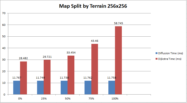
256x256	256	65.31	65536	68.01
512x512	512	140.52	262144	277.07
1024x1024	1024	399.74	1048576	1146.38
2048x2048	2048	1745.79	4194304	4954.72

Iterations and time for varying grid sizes

As we can see when each node has an equal cost the parallel version only takes n iterations for an nxn grid but take n*n iterations for the sequential version. However as we can see if we were to introduce terrain costs the parallel version would likely take longer due to the frontier set where as the sequential version will always take n*n iterations where a path exists.