Parallel Diffusion vs Sequential Dijkstra

Both the parallel diffusion and sequential dijkstra implementations have been run on a range of 6 different maps. In each case the time to find a path and the number of nodes in the path have been recorded.

Each map is made up for a 32x32 grid where each tile has a varying terrain cost associated with it. In each case the source node is the top left corner and the goal node is the bottom left.

Map 1

Map 1 was the simplest of the maps containing no obstacles or costly terrain. In both the diffusion and dijkstra applications each found the same path; which in this case was to simply move directly from the start to the goal with a path length of 32 nodes. However diffusion was able to do this approximately 80% quicker taking only 0.18ms compared to 0.97ms for dijkstra.

Diffusion Path

Dijkstra path

Map 2

Map 2 contains some more obstacles and varying terrain we have a small 'beach' with a lake in the middle and river with a bridge in the centre. 

Of all the maps that were tested this provided the greatest variant in path length between the two implementations. Surprisingly the diffusion implementation found a shorter path traversing only 39 nodes to reach the destination compared to the 49 taken by dijkstra. The reason for this is that the diffusion implementation chooses to move over the terrain by walking across the beach and going straight through the river whereas dijkstra chooses to take the bridge across and avoid getting wet. 

Again diffusion was able to find the path quicker taking only 0.23ms compared to 1.01ms for dijkstra.

72.2% of people asked felt that diffusion provided a more realistic path compared to dijkstra

Diffusion Path

Dijkstra Path

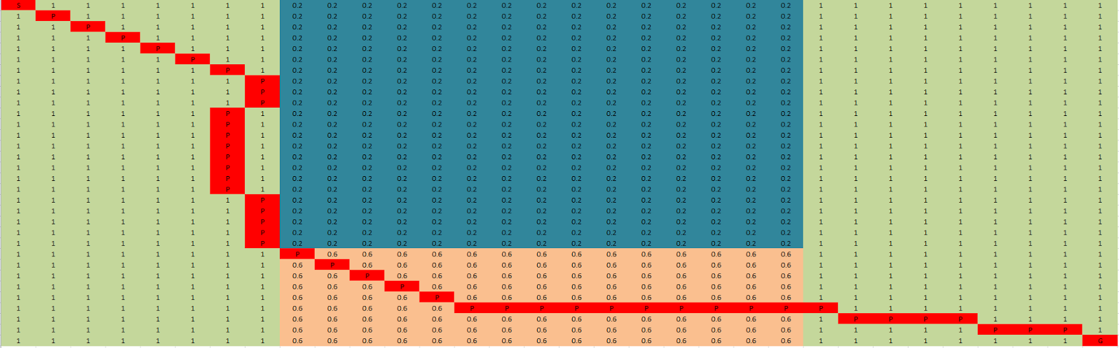
Map 3

Map 3 adds some more terrain and obstacles to the map covering approximately 50% of all the nodes.

Diffusion was able to find the shorter path again by choosing to walk across the beach in the centre to reach the goal, whereas dijkstra choose to avoid it resulting in a longer path traversing 41 nodes compared to diffusions 38.

Diffusion was also able to find the path quicker taking only 0.22ms compared to 1.05ms for dijkstra.

72.2% of people asked felt that diffusion provided a more realistic path compared to dijkstra

Diffusion Path

Dijkstra Path

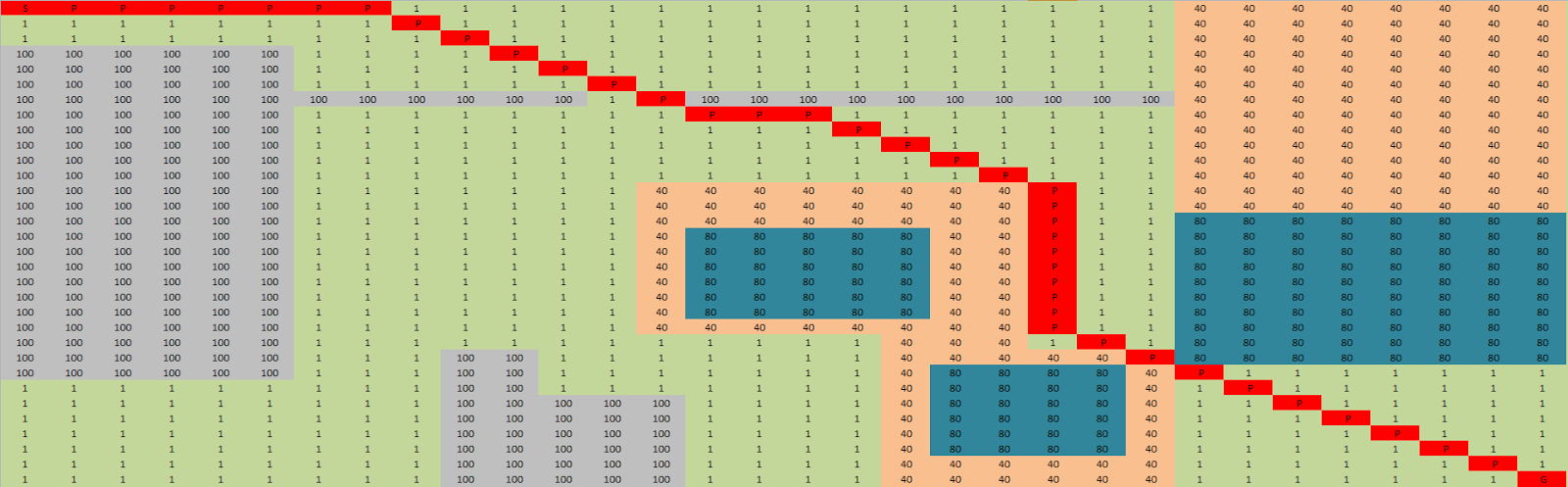
Map 4

Map 4 was the most complex of all the maps that were tested providing a maze like structure for the implementations to solve. Interestingly both were able to find pretty much the same path traversing 61 nodes to reach the goal. 

In this example dijkstra was actually able to find the path quicker than diffusion, however this is believed to be down to the specific implementation of diffusion.

66.7% of people asked felt that dijkstra provided a more realistic path compared to diffusion

Diffusion Path

Dijkstra Path

Map 5

In map 5 we test what happens when the goal is inaccessible. In both cases a path could not be found from the start to the goal. Interestingly again dijkstra was able to find that no path exists quicker than diffusion, however this is due to the nature of the diffusion implementation itself. 

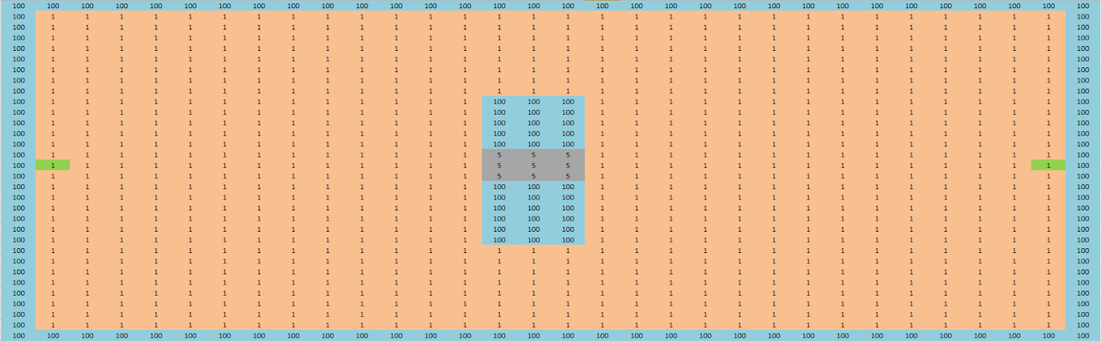
Map 6

In map 6 we test what happens when we must move through a set of terrain.

Both diffusion and dijkstra chose to move over the less costly of the two terrain options and both found a path in which they traverse 47 nodes to reach the goal, however looking at the images below we can see they actually take very different paths.

Diffusion was able to find a path quicker taking only 0.18ms compare to 0.95ms for dijkstra.

50% of people asked felt that diffusion provided a more realistic path compared to dijkstra

diffusion path

dijkstra path

Meetings: Monday 27th January

Until the new GPU arrives the aim is to continue writing up the methodology and the experiments that have been carried out with the current complete applications. Discussed ways that experiments should be presented and how the results should be analysed.

Meetings: Monday 20/01/14

Discussed the work that has been carried out during the winter break.

During the holidays i applied for an academic hardware donation from Nvidia, they have kindly agreed to donate a Tesla K40 to help with the project. This will provide the power of dynamic parallelism which should simplify the parallel Dijkstra application and provide a significant speed up. However the card will not be arriving until February which adds an extra time pressure to the project.

Currently have the following applications completed

• Sequential Diffusion
• Parallel Diffusion
• Sequential Dijkstra
• Sequential A* 
• Parallel Euclidean Distance

Until the card arrives the time will be spent writing up the methodology and the implementation for the applications which have been completed. Once the card has arrived the planned tests can be carried out and the results written up. 

Technical Work: Sequential Dijkstra

One of the pathfinding algorithms that i am aiming to compare against the parallel diffusion implementation is a sequential and parallel implementation of Dijkstra. This post will provide a background to Dijkstra's algorithm and an overview of the sequential implementation.

Background

Dijkstra's algorithim was first presented by Edsger Dijkstra in 1959 as a path finding algorithm that solves the single-source shortest path problem for a non-negative weighted graph. Nodes in the graph can represent either a 2-dimensional grid or points in 3D space. In many examples it is often used to find paths between connected cities where each city is represented as a node in the graph and each edge is a road with an associated cost. For a given source node dijkstra is able to find the lowest cost path between that node and every other node in the graph.

Non-negative weighted graph of connected cities.

The algorithm itself works by assigning a distance value to each node in the graph,  setting the value for our source node to zero and every other node to infinity. Initially we mark all nodes as unvisited and store them in a priority queue called the unvisited set. For our current source node we look at all of its unvisited neighbours and calculate the distance from our current node to the neighbouring node. For example, in figure 1 above if our current node was Tranent and we were looking at neighbour Musselburgh our distance would be 4. If this distance is less than our previous shortest path we add our current node to a shortest path tree which we can later use to backtrack a path to the source node. Once we have looked at all the neighbouring nodes we remove our current node from the unvisited set and it will not be checked again. Next we set our current node to the node with the smallest distance in the unvisited set and repeat the process with this nodes neighbours until all the nodes have been visited. At this point our shortest path graph will now contain all of the lowest cost paths from our source node to every other node, we can then perform a depth-first search over this graph to find a path from any node to the source.

Sequential Implementation

Our sequential implementation initially reads in a map from a .CSV file containing the costs of each tile in a 2D grid.

Example cost Grid

From this we build up a non-negative weighted graph of connected nodes which is stored in a 2 dimensional vector. Each node in the graph has an associated id, cost and list of its connected neighbours. A node is connected to other nodes based on the 8 surrounding nodes in the cost grid, for each neighbour diagonal to a node its cost is increased slightly. 

Once we have the node graph set up we are able to run our dijkstra algorithm on the graph. Our method takes in the x and y co-ordinates of the source node, a vector that will be used to store the minimum distance of each node to the source and a vector containing the previous position of the node closest to the source. 

Run the Dijkstra algorithm

Within the dijkstra method we create a priority queue to store all our unvisited nodes, we use a priority queue as it allows easy insertion and deletion of nodes and keeps our nodes ordered with the lowest cost node first in the queue. We then add our source node to the queue setting its initial cost to zero. 

While there a still nodes remaining unvisited in the queue we perform the following actions. 

1. Remove the node with the lowest cost from the queue.
2. Visit each of the nodes neighbours
• Calculate the cost of passing through this neighbour
• If this cost is less than our previously calculated cost
• Set the new cost to our new minimum cost
• set the parent of this neighbour to the current node being checked
• add the neighbour to the queue with the new calculated cost
3. Repeat step 1 if queue is not empty.

Once the queue is empty all of our nodes will have been visited and our previous vector will contain a shortest path tree for all of the nodes to the source. At this stage we can backtrack a path from any node to the source node. 

Our backtrack method takes a given goal node and using the shortest path tree backtracks through each of the nodes parent nodes adding them to a list until it reaches the original source node. 

At this point we now have a list containing all the nodes in a path between the original source node and the specified goal, this is then written to a .csv file so that we may view the path.

Examples

In each of these examples we read in a 32x32 cost grid to create our node graph from and perform our pathfinding to find a path between two points in the grid. The length of a path is defined as the number of nodes in the path and the cost of a path is the total cost of all the nodes.

In the first example above we have essentially an empty cost grid where every tiles value is 1 and we are trying to find a path between the two green points.

 

Above we can see that as would typically be expected the best and shortest path between the two points would be to move in a straight line. the length of the path is 30 and the cost of this path is 29. 

Above we have added a small lake into the center of our map, the cost of passing through a tile with water in it is 100.

As we can see our path has avoided the water, choosing instead to simply go around rather than through. This is due to the fact that moving through the water would incur a large cost and as such is not the shortest path. The length of this path is 30 and the cost is 43 (Moving diagonally has an additional cost).

This time we have added an old rickety bridge across the water with a cost of 25 to cross. 

While costing less to cross than water, crossing the old bridge would still not be the shortest path between our two points and as such our path has chosen to avoid it and go around the water. This path has a length of 30 and a cost of 43.

Our bridge has been upgraded to a super strong concrete bridge made by the finest engineers and now only has a cost of 5 to cross. 

As our bridge is now more stable and has a lower cost to cross, the shortest path between our two points is now to take the bridge rather than going around and as such our path length is 30 with a cost of 41.