Discussed the poster presentation and what needs to be included in the poster. The aim is to have an initial draft by Monday 31st March.
Also need to revise the initial questions outlined during the background. Possible questions are.
1. Find a suitable algorithm for path finding on the GPU.
2. Quantify in terms of
a) speed
b) Layout of path - scalability
c) trade-off : Speed vs Path style
3. What contributes to the GPU - Mapping of algorithms to the GPU
Also need a section for contributions.
Monday, 24 March 2014
Monday, 17 March 2014
Meetings: Monday 17th March
Discussed the results obtained from last weeks experiments and concluded that all the implementation, results and testing have all been completed. The remainder of the project will be focused on the write up and the poster session.
Discussed that it should be possible to use the coursework for computational intelligence to show a robot moving through the maze using collaborative diffusion.
Discussed that it should be possible to use the coursework for computational intelligence to show a robot moving through the maze using collaborative diffusion.
Thursday, 13 March 2014
Parallel Dijkstra
 |
| Map 1 |
 |
| Map 2 |
 |
| Map 3 |
 |
| Map 4 |
 |
| Map 5 |
 |
| Map 6 |
The parallel dijkstra application has been tested on the original 5 maps used on the sequential dijkstra and the diffusion applications. For each map the parallel version found the same path as the sequential version.
|
Map
|
Parallel
(ms)
|
Sequential
(ms)
|
|
1
|
8.42
|
0.97
|
|
2
|
33.82
|
1.01
|
|
3
|
40.78
|
1.05
|
|
4
|
55.87
|
1.00
|
|
5
|
18.58
|
0.64
|
|
6
|
51.91
|
0.95
|
Time for each map
Looking at the times taken for each map we can see quite a large difference between the parallel and sequential times. Even between the differing maps there is a large variation for just the parallel times, whereas the sequential times remain fairly consistent at around 1ms.
This is due to main while loop of the dijkstra application, where loop until the queue is empty and all nodes have been evaluated.
|
Map
|
Parallel
|
Sequential
|
|
1
|
32
|
1024
|
|
2
|
132
|
1024
|
|
3
|
159
|
1024
|
|
4
|
219
|
1024
|
|
5
|
72
|
701
|
|
6
|
203
|
1024
|
Iterations to evaluate all nodes in queue
Looking at the number of iterations needed in the sequential version we can see that it remains pretty much consistent taking 1024 iterations to evaluate each node in the queue, interestingly this is the total number of nodes added to the queue as we have 32*32 nodes and we evaluate each one. (Note: map 5 we only add 701 nodes to the queue as a number of nodes are blocked.)
However looking at the parallel version the number of iterations jumps between 32 and 219 for the differing map sizes. This is due to the frontier function and the way in which the parallel application works.
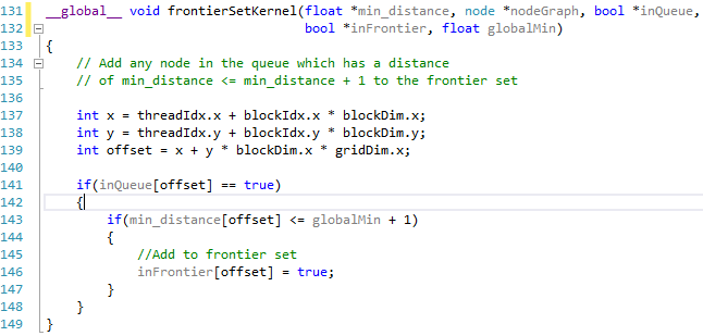
The parallel application determines which nodes in the queue can be settled at the same time and adds them to the frontier set. Any node in the queue which has a distance of less than the minimum distance + 1 will be added to the queue.
In each of the maps a lot of nodes have varying costs, these varying costs between neighbours will effect which nodes in the queue can be added to the frontier set and settled at the same time, the more variation between nodes the more iterations it will take to find the path. In each instance the worst case should be 1024 iterations for the 32x32 grid.
This also helps to explain why we see a speed up for the larger graph sizes, while the CPU is able to process 1024 iterations faster than the GPU can handle 32; for the large graph sizes the sequential version will need to take nxn iterations so for a 2048x2048 grid this would be 4,194,304 iterations.
|
Map
|
Parallel
|
Parallel
Time
|
Sequential
|
Sequential
Time
|
|
32x32
|
32
|
8.34
|
1024
|
1
|
|
64x64
|
64
|
16.37
|
4096
|
3.8
|
|
128x128
|
128
|
32.52
|
16384
|
16.2
|
|
256x256
|
256
|
65.31
|
65536
|
68.01
|
|
512x512
|
512
|
140.52
|
262144
|
277.07
|
|
1024x1024
|
1024
|
399.74
|
1048576
|
1146.38
|
|
2048x2048
|
2048
|
1745.79
|
4194304
|
4954.72
|
Iterations and time for varying grid sizes
As we can see when each node has an equal cost the parallel version only takes n iterations for an nxn grid but take n*n iterations for the sequential version. However as we can see if we were to introduce terrain costs the parallel version would likely take longer due to the frontier set where as the sequential version will always take n*n iterations where a path exists.
Monday, 10 March 2014
Meetings: Monday 10th March 2014
Discussed the results from the following set of tests and concluded that there is not much other work that can be done on this area at this time. http://10004794-honours-project.blogspot.co.uk/2014/03/streams-vs-device-functions-2.html
All that is really left to do is test the parallel implementation on the 5 test maps and then continue writing up the results. This week will most likely be the final week of coding for the project.
All that is really left to do is test the parallel implementation on the 5 test maps and then continue writing up the results. This week will most likely be the final week of coding for the project.
Wednesday, 5 March 2014
Streams vs Device Functions 2
In the previous post we looked at using device functions and evaluating each of the neighbours sequentially compared to using streams and evaluating each of the neighbours concurrently.
Interestingly we found that performing the check sequentially was actually faster than using streams, this post attempts to determine why this is.

Interestingly we found that performing the check sequentially was actually faster than using streams, this post attempts to determine why this is.
Map
|
Sequential Time
|
Device functions
|
Streams
|
32x32
|
1
|
8.341714
|
21.75491
|
64x64
|
3.8
|
16.37582
|
47.9231
|
128x128
|
16.2
|
32.52248
|
133.1749
|
256x256
|
68.01
|
65.31222
|
409.7781
|
512x512
|
277.07
|
140.5209
|
19658.81
|
1024x1024
|
1146.38
|
399.7442
|
144157.2
|
2048x2048
|
4954.72
|
1745.794
|
462554.9
|
Device Functions vs Streams
 |
| Evaluate Neighbours Device Function |
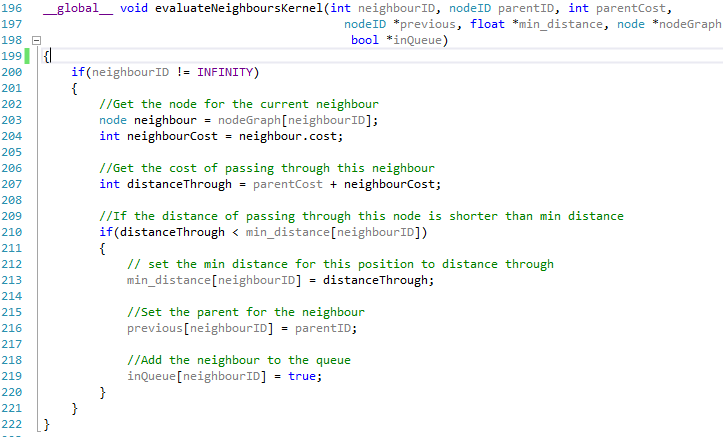 |
| Evaluate Neighbours Kernel |
Looking at the code snippets above they are both almost identical, the only real difference is that one is tagged with the __device__ keyword while the other is tagged with __global__, however this seems to make a big difference.
Map
|
Device Function
|
Create streams
|
Kernel with Streams
|
Kernel without streams
|
32x32
|
0.014075
|
0.017313
|
0.284529
|
0.262266
|
64x64
|
0.014052
|
0.017732
|
0.315197
|
0.297716
|
128x128
|
0.014728
|
0.018648
|
0.308442
|
0.400251
|
Time for different methods of evaluating neighbours
When we call a device function from within a thread we are not actually creating a new parallel block and thread to handle the process we are simply just calling a function in the same manner we could from the host. However when we use a kernel to handle the evaluation we need to launch a block and thread to handle the process, when using streams to launch the kernels concurrently we also have an extra overhead of having to create the streams.
Looking at the graph above we can see that we can call the device function to evaluate all 8 of our nodes neighbours quicker than we can create 8 streams to handle the neighbours. On top of the stream creating we also have to launch 8 kernels creating 8 blocks and threads to process the neighbors, this process in itself is extremely slow taking almost 18X longer than it does to call our device function.
Interestingly however it appears that using streams is potentially faster than not using streams, however this would really need to be tested for more graph sizes to get a fair results, this was not possible at the time due to errors in the timing code for large graph sizes.
The next change that was attempted involved each node storing a list of its neighbours in global memory on the device. In doing this it meant that it would be possible to call a single kernel which could be used to evaluate all of the 8 neighbours at the same time rather than calling an individual kernel for each neighbour as is needed when storing the nodes neighbours in local memory.

The next change that was attempted involved each node storing a list of its neighbours in global memory on the device. In doing this it meant that it would be possible to call a single kernel which could be used to evaluate all of the 8 neighbours at the same time rather than calling an individual kernel for each neighbour as is needed when storing the nodes neighbours in local memory.
 | ||||||||||||||||||||||||||||||||||||||||||||||||||||||||||||||||
| Evaluate all neighbours kernel
This resulted in a large speed up when compared to calling an individual kernel for each neighbour when using streams, however it is still slower than calling device functions. There was very little difference between calling the device functions when storing the neighbours in local memory compared to global memory.
|
Subscribe to:
Comments (Atom)