Iteration
|
Nodes In Frontier
|
0
|
1
|
1
|
3
|
2
|
5
|
3
|
7
|
4
|
9
|
5
|
11
|
6
|
13
|
7
|
15
|
8
|
17
|
9
|
19
|
10
|
21
|
11
|
23
|
12
|
25
|
13
|
27
|
14
|
29
|
15
|
31
|
16
|
33
|
17
|
35
|
18
|
37
|
19
|
39
|
20
|
41
|
21
|
43
|
22
|
45
|
23
|
47
|
24
|
49
|
25
|
51
|
26
|
53
|
27
|
55
|
28
|
57
|
29
|
59
|
30
|
61
|
31
|
63
|
Monday, 21 July 2014
Nodes added to the frontier set each iteration
number of nodes added to frontier set each iteration increase by 2, ascending in odd numbers to n + n -1 where n is the size of the grid. the sum of the nodes added each iteration for all iterations is equal to n*n.

Monday, 14 July 2014
Parallel Dijkstra

|
Map
|
Time
|
|
32X32
|
3.46784
|
|
64X64
|
6.455913
|
|
128X128
|
13.38988
|
|
256X256
|
28.1704
|
|
512X512
|
72.76363
|
|
1024X1024
|
278.0663
|
|
2048X2048
|
1729.728
|
|
4096X4096
|
10725.9
|
|
8192X8192
|
80471.69
|
Internship Plan - 14/07/14
- Explore path search algorithms using CUDA Dynamic Parallelism
- Cut down Honours Project
- Extend Tests
- Weighted vs Non-Weighted
- Fine grained dynamic parallelism support for Dijkstra
- Do more practical work
- Examine Frontier Sets
- Parallelise A*
- Compare to Ortega-Arranz Implementation
- Read Requirements of Journals
- Plan out what the paper will look like
Possible Journals and Conferences
- High Performance Computing & Simulation
- Concurrency and Computation, Practice and Experience
- GPU Gems
- GTC
Thursday, 10 April 2014
Poster Presentation 9th April 2014

The video below is a small demo which shows the difference in paths between diffusion and dijkstra. The green paths represent diffusion while the purple paths represent dijkstra.
Monday, 24 March 2014
Meetings: Monday 24th March 2014
Discussed the poster presentation and what needs to be included in the poster. The aim is to have an initial draft by Monday 31st March.
Also need to revise the initial questions outlined during the background. Possible questions are.
1. Find a suitable algorithm for path finding on the GPU.
2. Quantify in terms of
a) speed
b) Layout of path - scalability
c) trade-off : Speed vs Path style
3. What contributes to the GPU - Mapping of algorithms to the GPU
Also need a section for contributions.
Also need to revise the initial questions outlined during the background. Possible questions are.
1. Find a suitable algorithm for path finding on the GPU.
2. Quantify in terms of
a) speed
b) Layout of path - scalability
c) trade-off : Speed vs Path style
3. What contributes to the GPU - Mapping of algorithms to the GPU
Also need a section for contributions.
Monday, 17 March 2014
Meetings: Monday 17th March
Discussed the results obtained from last weeks experiments and concluded that all the implementation, results and testing have all been completed. The remainder of the project will be focused on the write up and the poster session.
Discussed that it should be possible to use the coursework for computational intelligence to show a robot moving through the maze using collaborative diffusion.
Discussed that it should be possible to use the coursework for computational intelligence to show a robot moving through the maze using collaborative diffusion.
Thursday, 13 March 2014
Parallel Dijkstra
 |
| Map 1 |
 |
| Map 2 |
 |
| Map 3 |
 |
| Map 4 |
 |
| Map 5 |
 |
| Map 6 |
The parallel dijkstra application has been tested on the original 5 maps used on the sequential dijkstra and the diffusion applications. For each map the parallel version found the same path as the sequential version.
|
Map
|
Parallel
(ms)
|
Sequential
(ms)
|
|
1
|
8.42
|
0.97
|
|
2
|
33.82
|
1.01
|
|
3
|
40.78
|
1.05
|
|
4
|
55.87
|
1.00
|
|
5
|
18.58
|
0.64
|
|
6
|
51.91
|
0.95
|
Time for each map
Looking at the times taken for each map we can see quite a large difference between the parallel and sequential times. Even between the differing maps there is a large variation for just the parallel times, whereas the sequential times remain fairly consistent at around 1ms.
This is due to main while loop of the dijkstra application, where loop until the queue is empty and all nodes have been evaluated.
|
Map
|
Parallel
|
Sequential
|
|
1
|
32
|
1024
|
|
2
|
132
|
1024
|
|
3
|
159
|
1024
|
|
4
|
219
|
1024
|
|
5
|
72
|
701
|
|
6
|
203
|
1024
|
Iterations to evaluate all nodes in queue
Looking at the number of iterations needed in the sequential version we can see that it remains pretty much consistent taking 1024 iterations to evaluate each node in the queue, interestingly this is the total number of nodes added to the queue as we have 32*32 nodes and we evaluate each one. (Note: map 5 we only add 701 nodes to the queue as a number of nodes are blocked.)
However looking at the parallel version the number of iterations jumps between 32 and 219 for the differing map sizes. This is due to the frontier function and the way in which the parallel application works.
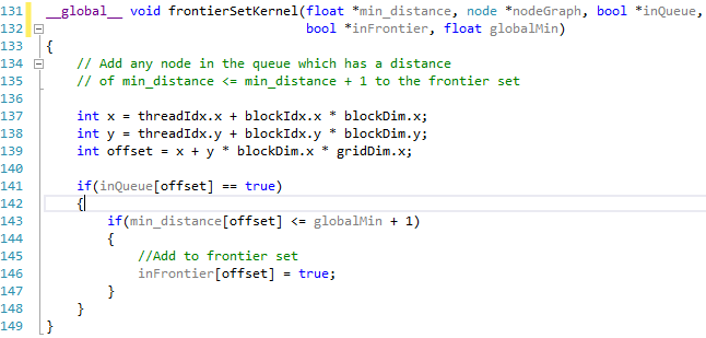
The parallel application determines which nodes in the queue can be settled at the same time and adds them to the frontier set. Any node in the queue which has a distance of less than the minimum distance + 1 will be added to the queue.
In each of the maps a lot of nodes have varying costs, these varying costs between neighbours will effect which nodes in the queue can be added to the frontier set and settled at the same time, the more variation between nodes the more iterations it will take to find the path. In each instance the worst case should be 1024 iterations for the 32x32 grid.
This also helps to explain why we see a speed up for the larger graph sizes, while the CPU is able to process 1024 iterations faster than the GPU can handle 32; for the large graph sizes the sequential version will need to take nxn iterations so for a 2048x2048 grid this would be 4,194,304 iterations.
|
Map
|
Parallel
|
Parallel
Time
|
Sequential
|
Sequential
Time
|
|
32x32
|
32
|
8.34
|
1024
|
1
|
|
64x64
|
64
|
16.37
|
4096
|
3.8
|
|
128x128
|
128
|
32.52
|
16384
|
16.2
|
|
256x256
|
256
|
65.31
|
65536
|
68.01
|
|
512x512
|
512
|
140.52
|
262144
|
277.07
|
|
1024x1024
|
1024
|
399.74
|
1048576
|
1146.38
|
|
2048x2048
|
2048
|
1745.79
|
4194304
|
4954.72
|
Iterations and time for varying grid sizes
As we can see when each node has an equal cost the parallel version only takes n iterations for an nxn grid but take n*n iterations for the sequential version. However as we can see if we were to introduce terrain costs the parallel version would likely take longer due to the frontier set where as the sequential version will always take n*n iterations where a path exists.
Subscribe to:
Posts (Atom)