Scattered Terrain: Diffusion vs Dijkstra

Both diffusion and dijkstra have been tested on larger maps with varying terrain. These maps are 256X256 and each has a different percentage of the map covered with terrain. Terrain costs are represented by a random value between 1 and 10 for dijkstra and 0 and 1 for diffusion. In the images bellow terrain is represented by the red areas. Paths are represented by the blue tiles.

0% Terrain

25% Scattered Terrain

50% Scattered Terrain

75% Scattered Terrain

100% Scattered Terrain

25% Centred Terrain

50% Centred Terrain

75% Centred Terrain

100% Centred Terrain

25% Split Terrain

50% Split Terrain

75% Split Terrain

100% Split Terrain

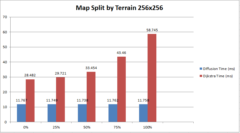
Looking at the graphs above it is interesting to see that for all the maps diffusion performs the same regardless of how much terrain there is in the map and where the terrain is in the map taking 11ms to diffuse the values and find path.

Looking at Dijkstra however for each of the sets of maps we can see that as the amount of terrain in the map increases so does the time it takes to find a path.

Looking at the line graph above we can also see that the position of the terrain in the maps also effects the time taken by dijkstra to find the path. the more scattered the terrain the longer Dijkstra takes to find a path? although this could be due to the fact that there is less terrain? - more likely this?

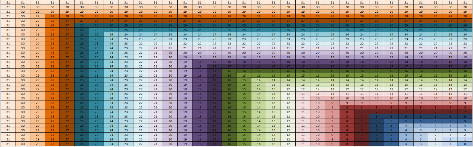
Visualization of nodes added to frontier set

Each colour represents the iteration of the outer loop that the node was added to the frontier set.

Tests to run

Run both dijkstra and diffusion for maps with varying terrain, use larger maps with different portions covered with terrain. i.e 25% 50% 75% and have terrain spread out vs grouped together See how this effects the time taken and the nodes added to the frontier set.

Run each for an average of 10 times,

create the maps and store them in a .CSV file so the same maps can be used each time.

Nodes added to the frontier set each iteration

number of nodes added to frontier set each iteration increase by 2, ascending in odd numbers to n + n -1 where n is the size of the grid. the sum of the nodes added each iteration for all iterations is equal to n*n.

Iteration	Nodes In Frontier
0	1
1	3
2	5
3	7
4	9
5	11
6	13
7	15
8	17
9	19
10	21
11	23
12	25
13	27
14	29
15	31
16	33
17	35
18	37
19	39
20	41
21	43
22	45
23	47
24	49
25	51
26	53
27	55
28	57
29	59
30	61
31	63

Parallel Dijkstra

Map	Time
32X32	3.46784
64X64	6.455913
128X128	13.38988
256X256	28.1704
512X512	72.76363
1024X1024	278.0663
2048X2048	1729.728
4096X4096	10725.9
8192X8192	80471.69

Internship Plan - 14/07/14

1. Explore path search algorithms using CUDA Dynamic Parallelism 
1. Cut down Honours Project
2. Extend Tests
3. Weighted vs Non-Weighted
2. Fine grained dynamic parallelism support for Dijkstra
1. Do more practical work
3. Examine Frontier Sets
4. Parallelise A*
5. Compare to Ortega-Arranz Implementation
6. Read Requirements of Journals
7. Plan out what the paper will look like

Possible Journals and Conferences

1. High Performance Computing & Simulation
2. Concurrency and Computation, Practice and Experience
3. GPU Gems
4. GTC

Poster Presentation 9th April 2014

The video below is a small demo which shows the difference in paths between diffusion and dijkstra. The green paths represent diffusion while the purple paths represent dijkstra.